5 Stochastic Layer
5.1 Description
The stochastic layer is populated with failure probabilities or failure probability distributions associated with basic events (in the event tree linking approach, functional events also can be associated with such a distribution). Probability distributions are described by (stochastic) expressions, which are terms, according to the terminology of Chapter 3. These expressions may depend on parameters (variables), so the stochastic layer can be seen a set of stochastic equations.
Stochastic equations associated with basic events actually play two roles:
- They are applied to calculate probability distributions of each basic event, i.e., for a given mission time \(t\), the probability \(Q(t)\) that the given basic event occurs before \(t\). The probability distribution associated with a basic event is typically a negative exponential distribution of parameter \(\lambda\):
Note that, for the sake of the clarity, the Model Exchange Format represents explicitly the mission time as a parameter of a special type.
- Parameters are sometimes not known with certainty. Sensitivity analyses, such as Monte-Carlo simulations, are thus performed to study the change in risk due to this uncertainty. Expressions, therefore, are used to describe distributions of parameters. Typically, the parameter \(\lambda\) of a negative exponential distribution will be itself distributed according to a lognormal law of mean 0.001 and error factor 3.
Stochastic expressions are made of the following elements:
- Boolean and numerical constants
- Stochastic variables, i.e., parameters, including the special variable to represent the mission time
- Boolean and arithmetic operations (sums, differences, products, etc.)
- Built-in expressions that can be seen as macro-expressions that are used to simplify and shorten the writing of probability distributions (exponential, Weibull, etc.)
- Primitives to generate numbers at pseudo-random according to some probability distribution. The base primitive makes it possible to generate random deviates with a uniform probability distribution. Several other primitives are derived from this one to generate random deviates with normal, lognormal, or other distributions. Moreover, it is possible to define discrete distributions “by hand” through the notion of histogram.
- Directives to test the status of initial and functional events
Listing 5.1 presents the RNC schema for the constructs of the stochastic layer. Note that, conversely to variables (events) of the Fault Tree layer, parameters have to be defined (there is no equivalent to Basic Events).
expression =
  constant
  | parameter
  | operation
  | built-in
  | random-deviate
  | test-event

operation =
  numerical-operation | Boolean-operation | conditional-operation

built-in = exponential | GLM | Weibull | periodic-test | extern-function

random-deviate =
  uniform-deviate
  | normal-deviate
  | lognormal-deviate
  | gamma-deviate
  | beta-deviate
  | histogram

test-event = test-initiating-event | test-functional-event
The XML representation of the stochastic layer just reflects these different constructs.
parameter-definition =
  element define-parameter {
    name,
    role?,
    attribute unit { units }?,
    label?,
    attributes?,
    expression
  }

parameter =
  element parameter {
    reference,
    attribute unit { units }?
  }
  | element system-mission-time {
      attribute unit { units }?
    }

units =
  "bool"
  | "int"
  | "float"
  | "hours"
  | "hours-1"
  | "years"
  | "years-1"
  | "fit"
  | "demands"

constant = bool | int | float

bool =
  element bool {
    attribute value { Boolean-value }
  }

int =
  element int {
    attribute value { xsd:integer }
  }

float =
  element float {
    attribute value { xsd:double }
  }
Operations, built-ins, and random deviates will be described in the following sections.
We believe that the formalism to define stochastic equations should be as large and as open as possible for at least two reasons: first, available tools already propose a large set of distributions; second, this is an easy and interesting way to widen the spectrum of PSA. The Model Exchange Format proposes a panoply of Boolean and arithmetic operators. More operations can be added on demand. A major step would be to introduce some algorithmic concepts like loops and functions. At this stage, it does seem useful to introduce such advanced concepts in the Model Exchange Format.
5.2 Operations
5.2.1 Numerical Operation
Table 5.1 gives the list of arithmetic operators proposed by the Model Exchange Format. Their XML representation is given in Listing 5.3.
| Operator | #arguments | Semantics |
|---|---|---|
| neg | 1 | unary minus |
| add | >1 | addition |
| sub | >1 | subtraction |
| mul | >1 | multiplication |
| div | >1 | division |
| pi | 0 | 3.1415926535... |
| abs | 1 | absolute value |
| acos | 1 | arc cosine of the argument in radians |
| asin | 1 | arc sine of the argument in radians |
| atan | 1 | arc tangent of the argument in radians |
| cos | 1 | cosine |
| cosh | 1 | hyperbolic cosine |
| exp | 1 | exponential |
| log | 1 | (Napierian) logarithm |
| log10 | 1 | decimal logarithm |
| mod | 2 | modulo |
| pow | 2 | power |
| sin | 1 | sine |
| sinh | 1 | hyperbolic sine |
| tan | 1 | tangent |
| tanh | 1 | hyperbolic tangent |
| sqrt | 1 | square root |
| ceil | 1 | first integer not less than the argument |
| floor | 1 | first integer not greater than the argument |
| min | >1 | minimum |
| max | >1 | maximum |
| mean | >1 | mean |
numerical-operation =
  element neg { expression }
  | element add { expression+ }
  | element sub { expression+ }
  | element mul { expression+ }
  | element div { expression+ }
  | element pi { empty }
  | element abs { expression }
  | element acos { expression }
  | element asin { expression }
  | element atan { expression }
  | element cos { expression }
  | element cosh { expression }
  | element exp { expression }
  | element log { expression }
  | element log10 { expression }
  | element mod { expression, expression }
  | element pow { expression, expression }
  | element sin { expression }
  | element sinh { expression }
  | element tan { expression }
  | element tanh { expression }
  | element sqrt { expression }
  | element ceil { expression }
  | element floor { expression }
  | element min { expression+ }
  | element max { expression+ }
  | element mean { expression+ }
5.2.1.1 Example
Assume, for instance, we want to associate a negative exponential distribution with a failure rate \(\lambda = {1.23 \times 10^{-4}}h^{-1}\) to the basic event “pump-failure”. Using primitives defined above, we can encode explicitly such probability distribution as follows.
<define-basic-event name="pump-failure">
    <sub>
        <float value="1.0"/>
        <exp>
            <mul>
                <neg>
                    <parameter name="lambda"/>
                </neg>
                <system-mission-time/>
            </mul>
        </exp>
    </sub>
</define-basic-event>
<define-parameter name="lambda">
    <float value="1.23e-4"/>
</define-parameter>
5.2.2 Boolean Operations
Table 5.2 gives the list of Boolean operators proposed by the Model Exchange Format. Their XML representation is given in Listing 5.4.
| Operator | #arguments | Semantics |
|---|---|---|
| and | >1 | \(\land\) |
| or | >1 | \(\lor\) |
| not | 1 | \(\lnot\) |
| eq | 2 | \(=\) |
| df | 2 | \(\neq\) |
| lt | 2 | \(<\) |
| gt | 2 | \(>\) |
| leq | 2 | \(\leq\) |
| geq | 2 | \(\geq\) |
Boolean-operation =
  element not { expression }
  | element and { expression+ }
  | element or { expression+ }
  | element eq { expression, expression }
  | element df { expression, expression }
  | element lt { expression, expression }
  | element gt { expression, expression }
  | element leq { expression, expression }
  | element geq { expression, expression }
5.2.3 Conditional Operations
The Model Exchange Format proposes two conditional operations: an “if-then-else” operation and a “switch/case” operation. The latter is a list of pairs of expressions introduced by the tag “case”. The first expression of the pair should be a Boolean condition. If this condition is realized, then the second expression is evaluated, and its value returned. Otherwise, the next pair is considered.
The list ends with an expression in order to be sure that the switch has always a possible value. The XML representation for conditional operation is given in Listing 5.5.
conditional-operation = if-then-else-operation | switch-operation

if-then-else-operation =
  element ite { expression, expression, expression }

switch-operation = element switch { case-operation*, expression }

case-operation = element case { expression, expression }
5.2.3.1 Example
Assume, for instance, we want to give different values to the failure rate “lambda” depending on a global parameter “stress-level”:
"lambda"=1.0e-4/h if "stress-level"=1,
"lambda"=2.5e-4/h if "stress-level"=2, and finally
"lambda"=1.0e-3/h if "stress-level"=3.
The value of “stress-level” will be modified while walking along the sequences of event trees or depending on the initiating event. Using primitives defined so far, we can encode the definition of “lambda” as follows.
<define-parameter name="lambda">
    <switch>
        <case>
            <eq>
                <parameter name="stress-level"/>
                <int value="1"/>
            </eq>
            <float value="1.0e-4"/>
        </case>
        <case>
            <eq>
                <parameter name="stress-level"/>
                <int value="2"/>
            </eq>
            <float value="2.5e-4"/>
        </case>
        <float value="1.0e-3"/>
    </switch>
</define-parameter>
5.3 Built-Ins
5.3.1 Description
Built-ins can be seen as macro arithmetic expressions. They are mainly used to simplify the writing of probability distributions. A special built-in “extern-function” makes it possible to define externally calculated built-ins. As for arithmetic operators, more built-ins can be added on demand to the Model Exchange Format. Here follows a preliminary list of built-ins. Table 5.3 summarizes this preliminary list.
- Exponential with two parameters
- This built-in implements the negative exponential distribution. The two parameters are the hourly failure rate, usually called \(\lambda\), and the time \(t\).
- Exponential with four parameters (Generalized Life Model or GLM)
- This built-in generalizes the previous one. It makes it possible to take into account repairable components (through the hourly repairing rate \(\mu\)) and failures on demand (through the probability \(\gamma\) of such an event). It takes four parameters, \(\gamma\), the hourly failure rate \(\lambda\), \(\mu\), and the time \(t\) (in this order).
- Weibull
- This built-in implements the Weibull distribution. It takes four parameters: a scale parameter \(\alpha\), a shape parameter \(\beta\), a time shift \(t_0\), and the time \(t\) (in this order).
- Periodic test
- In several applications, it is of interest to introduce some specific distributions to describe periodically tested components. A further investigation is certainly necessary on this topic. We tentatively give here a candidate definition (that is extracted from one of the tools we considered).
The “periodic-test” built-in would take the following parameters (in order).
| \(\lambda\) | failure rate when the component is working. |
| \(\lambda*\) | failure rate when the component is tested. |
| \(\mu\) | repair rate (once the test showed that the component is failed). |
| \(\tau\) | delay between two consecutive tests. |
| \(\theta\) | delay before the first test. |
| \(\gamma\) | probability of failure due to the (beginning of the) test. |
| \(\pi\) | duration of the test. |
| \(x\) | indicator of the component availability during the test (1 available, 0 unavailable). |
| \(\sigma\) | test covering: probability that the test detects the failure, if any. |
| \(\omega\) | probability that the component is badly restarted after a test or a repair. |
| \(t\) | the mission time. |
Fig. 5.1 illustrates the meaning of the parameters \(\tau\), \(\theta\), and \(\pi\).
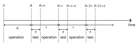
Fig. 5.1 Meaning of parameters \(\tau\), \(\theta\), and \(\pi\) of the “periodic-test” built-in
There are three phases in the behavior of the component. The first phase corresponds to the time from 0 to the date of the first test, i.e. \(\theta\). The second phase is the test phase. It spreads from times \(\theta + n\tau\) to \(\theta + n\tau + \pi\), with n any positive integer. The third phase is the functioning phase. It spreads from times \(\theta + n\tau + \pi\) to \(\theta + (n + 1)\tau\).
In the first phase, the distribution is a simple exponential law of parameter \(\lambda\).
The component may enter in the second phase in three states, either working, failed or in repair. In the latter case, the test is not performed. The Markov graphs for each of these cases are pictured in Fig. 5.2.
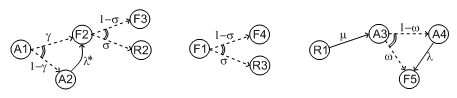
Fig. 5.2 Multi-phase Markov graph for the “periodic-test” built-in
Ai’s, Fi’s, Ri’s states correspond respectively to states where the component is available, failed, and in repair. Dashed lines correspond to immediate transitions. Initial states are respectively A1, F1, and R1.
The situation is simpler in the third phase. If the component enters available this phase, the distribution follows an exponential law of parameter \(\lambda\). If the component enters failed in this phase, it remains phase up to the next test. Finally, the Markov graph for the case where the component is in repair is the same as in the second phase.
The Model Exchange Format could also provide two simplified forms for the periodic test distribution.
- Periodic-test with 5 arguments
The first one takes five parameters: \(\lambda\), \(\mu\), \(\tau\), \(\theta\), and \(t\). In that case, the test is assumed to be instantaneous. Therefore, parameters \(\lambda*\) (the failure rate during the test) and \(x\) (indicator of the component availability during the test) are meaningless. There other parameters are set as follows.
- \(\gamma\) (the probability of failure due to the beginning of the test) is set to 0.
- \(\sigma\) (the probability that the test detects the failure, if any) is set to 1.
- \(\omega\) (the probability that the component is badly restarted after a test or a repair) is set to 0.
- Periodic-test with 4 arguments
- The second one takes only four parameters: \(\lambda\), \(\tau\), \(\theta\), and \(t\). The repair is assumed to be instantaneous (or equivalently the repair rate \(\mu = {+\infty}\)).
- Extern functions
- The Model Exchange Format should provide a mean to call extern functions. This makes it extensible and allows linking the PSA assessment tools with complex tools to calculate physical behavior (like fire propagation or gas dispersion). This call may take any number of arguments and return a single value at once (some interfacing glue can be used to handle the case where several values have to be returned). It has been also suggested that extern function calls take XML terms as input and output. This is probably the best way to handle communication between tools, but it would be far too complex to embed XML into stochastic expressions.
| Built-in | #arguments | Semantics |
|---|---|---|
| exponential | 2 | negative exponential distribution with hourly failure rate and time |
| GLM | 4 | negative exponential distribution with probability of failure on demand, hourly failure rate, hourly repair rate and time |
| Weibull | 4 | Weibull distribution with scale and shape parameters, a time shift and the time |
| periodic-test | 11, 5 or 4 | Distributions to describe periodically tested components |
| extern-function | any | call to an extern routine |
5.3.2 XML Representation
The RNC schema for the XML representation of built-ins is given in Listing 5.6.
exponential = element exponential { expression, expression }

GLM = element GLM { expression, expression, expression, expression }

Weibull = element Weibull { expression, expression, expression, expression }

periodic-test = element periodic-test { expression+ }

extern-function = element extern-function { name, expression* }
Positional versus Named Arguments
We adopted a positional definition of arguments. For instance, in the negative exponential distribution, we assumed that the failure rate is always the first argument, and the mission time is always the second. An alternative way would be to name arguments, i.e., to enclose them into tags explicating their role. For instance, the failure rate would be enclosed in a tag “failure-rate”, the mission time in a tag “time”, and so on. The problem with this second approach is that many additional tags must be defined, and it is not sure that it helps a lot the understanding of the built-ins. Nevertheless, we may switch to this approach if the experience shows that the first one proves to be confusing.
5.3.2.1 Example
The negative exponential distribution can be encoded as follows.
<define-basic-event name="pump-failure">
    <exponential>
        <parameter name="lambda"/>
        <system-mission-time/>
    </exponential>
</define-basic-event>
5.4 Primitive to Generate Random Deviates
5.4.1 Description
Primitives to generate random deviates are the real stochastic part of stochastic equations. They can be used in two ways: in a regular context they return a default value (typically their mean value). When used to perform Monte-Carlo simulations, they return a number drawn at pseudo-random according to their type. The Model Exchange Format includes two types of random deviates: built-in deviates like uniform, normal or lognormal, and histograms that are user defined discrete distributions. A preliminary list of distributions is summarized in Table 5.4. As for arithmetic operators and built-ins, this list can be extended on demand.
| Distribution | #arguments | Semantics |
|---|---|---|
| uniform-deviate | 2 | uniform distribution between a lower and an upper bounds |
| normal-deviate | 2 | normal (Gaussian) distribution defined by its mean and its standard deviation |
| lognormal-deviate | 3 or 2 | lognormal distribution defined by its mean, its error factor, and the confidence level of this error factor |
| gamma-deviate | 2 | gamma distributions defined by a shape and a scale factors |
| beta-deviate | 2 | beta distributions defined by two shape parameters \(\alpha\) and \(\beta\) |
| histograms | any | discrete distributions defined by means of a list of pairs |
- Uniform Deviates
- These primitives describe uniform distributions in a given range
defined by its lower- and upper-bounds.
The default value of a uniform deviate
is the mean of the range, i.e.,
(lower-bound + upper-bound)/2. - Normal Deviates
- These primitives describe normal distributions defined by their mean and their standard deviation (refer to a text book for a more detailed explanation). By default, the value of a normal distribution is its mean.
- Lognormal distribution
These primitives describe lognormal distributions defined by their mean \(E(x)\) and their error factor \(EF\). A random variable is distributed according to a lognormal distribution if its logarithm is distributed according to a normal distribution. If \(\mu\) and \(\sigma\) are respectively the mean and the standard deviation of the associated normal distribution (the variable’s natural logarithm), the probability density of the random variable is as follows.
\[f(x;\mu,\sigma) = \frac{1}{\sigma x \sqrt{2\pi}} \times \left[-\frac{1}{2}\left(\frac{\log x - \mu}{\sigma} \right)^2\right]\]Its mean, \(E(x)\), is defined as follows.
\[E(x) = \exp\left[\mu + \frac{\sigma^2}{2}\right]\]The error factor \(EF\) for confidence level \(\alpha\) is defined as follows:
\[\begin{split}EF_\alpha& = \sqrt{\frac{X_\alpha}{X_{1-\alpha}}} = \exp[z_\alpha\cdot\sigma]\\\end{split}\]Where \(X_\alpha\) is a left-tailed, upper bound corresponding to the \(\alpha\) percentile, and \(z_\alpha\) is the left-tailed z-score of the standard normal distribution for the \(\alpha\) confidence level. Note that one-sided limits do not form confidence intervals.
\[\begin{split}z_\alpha& = \sqrt{2} \cdot erf^{-1}(2\alpha - 1)\\ X_\alpha& = \exp[\mu + z_\alpha\cdot\sigma]\\ X_{0.50}& = e^\mu\end{split}\]For example, the error factor for a confidence level of \(0.95\):
\[\begin{split}z_{0.95}& = -z_{0.05} = 1.645\\ X_{0.05}& = \exp[\mu - 1.645\sigma]\\ X_{0.95}& = \exp[\mu + 1.645\sigma]\\ EF_{0.95}& = \sqrt{\frac{X_{0.95}}{X_{0.05}}} = \exp[1.645\sigma]\end{split}\]Once the mean and error factor are known for a certain confidence level, it is then possible to determine the distribution parameters of the lognormal law.
\[\begin{split}\sigma& = \frac{\log EF_\alpha}{z_\alpha}\\ \mu& = \log E(x) - \frac{\sigma^2}{2}\end{split}\]Alternatively, these parameters (\(\mu\), \(\sigma\)) of the underlying normal distribution can be supplied directly instead of the log-normal mean, error factor, and confidence level. These two parametrization schemes are distinguished by the number of parameters, i.e., 2 instead of 3.
- Gamma Deviates
These primitives describe Gamma distributions defined by their shape parameter k and their scale parameter \(\theta\). If \(k\) is an integer, then the distribution represents the sum of \(k\) exponentially distributed random variables, each of which has mean \(\theta\).
The probability density of the gamma distribution can be expressed in terms of the gamma function:
\[f(x) = x^{k-1} \frac{e^{-x/\theta}}{\theta^k \Gamma(k)}\]The default value of the gamma distribution is its mean, i.e., \(k\theta\).
- Beta Deviates
These primitives describe Beta distributions defined by two shape parameters \(\alpha\) and \(\beta\).
The probability density of the beta distribution can be expressed in terms of the B function:
\[\begin{split}f(x;\alpha,\beta)& = \frac{1}{B(\alpha,\beta)}x^{\alpha-1} (1 - x)^{\beta-1}\\ B(x, y)& = \int_{0}^{1} t^{x-1} (1 - t^{y-1}) dt\end{split}\]The default value of the beta distribution is its mean, i.e., \(\alpha/(\alpha + \beta)\).
- Histograms
Histograms are lists of pairs \((x_1, E_1), \ldots, (x_n, E_n)\), where the \(x_i\)‘s are numbers such that \(x_i < x_{i+1} \text{ for } i=1, \ldots, n-1\) and the \(E_i\)‘s are expressions.
The \(x_i\)‘s represent upper bounds of successive intervals. The lower bound of the first interval \(x_0\) is given apart.
The drawing of a value according to a histogram is a two-step process. First, a value \(z\) is drawn uniformly in the range \([x_0, x_n]\). Then, a value is drawn at random by means of the expression \(E_i\), where \(i\) is the index of the interval such that \(x_{i-1} < z \leq x_i\).
By default, the value of a histogram is its mean, i.e.,
\[\mathbf{E}(X) = \frac{1}{x_n - x_0} \times \sum_{i=1}^{n}(x_i - x_{i-1})\mathbf{E}(E_i)\]Both Cumulative Distribution Functions and Density Probability Distributions can be translated into histograms.
A Cumulative Distribution Function is a list of pairs \((p_1, v_1), \ldots, (p_n, v_n)\), where the \(p_i\)‘s are such that \(p_i < p_{i+1} \text{ for } i=1, \ldots, n \text{ and } p_n=1\). It differs from histograms in two ways. First, \(X\) axis values are normalized (to spread between 0 and 1); second, they are presented in a cumulative way. The histogram that corresponds to a Cumulative Distribution Function \((p_1, v_1), \ldots, (p_n, v_n)\) is the list of pairs \((x_1, v_1), \ldots, (x_n, v_n)\), with the initial value \(x_0 = 0, x_1 = p_1, \text{ and } x_i = p_i - p_{i-1} \text{ for all } i>1\).
A Discrete Probability Distribution is a list of pairs \((d_1, m_1), \ldots, (d_n, m_n)\). The \(d_i\)‘s are probability densities. However, they could be any kind of values. The \(m_i\)‘s are midpoints of intervals and are such that \(m_1 < m_2 < \ldots < m_n < 1\). The histogram that corresponds to a Discrete Probability Distribution \((d_1, m_1), \ldots, (d_n, m_n)\) is the list of pairs \((x_1, d_1), \ldots, (x_n, d_n)\), with the initial value \(x_0 = 0, x_1 = 2m_1, \text{ and } x_i = x_{i-1} + 2(m_i - x_{i-1})\).
5.4.2 XML Representation
The RNC schema for the XML representation of random deviates is given
uniform-deviate = element uniform-deviate { expression, expression }

normal-deviate = element normal-deviate { expression, expression }

lognormal-deviate =
  element lognormal-deviate { expression, expression, expression? }

gamma-deviate = element gamma-deviate { expression, expression }

beta-deviate = element beta-deviate { expression, expression }

histogram = element histogram { expression, bin+ }

bin = element bin { expression, expression }
5.4.2.1 Example
Assume that the parameter “lambda” of a negative exponential distribution is distributed according to a lognormal distribution of mean 0.001 and error factor 3 for a confidence level of 95%. The parameter “lambda” is then defined as follows.
<define-parameter name="lambda">
    <lognormal-deviate>
        <float value="0.001"/>
        <float value="3"/>
        <float value="0.95"/>
    </lognormal-deviate>
</define-parameter>
5.4.2.2 Example
Assume that the parameter “lambda” has been sampled outside of the model and is distributed according to the following histogram.

The XML encoding for “lambda” is as follows.
<define-parameter name="lambda">
    <histogram>
        <float value="100"/>
        <bin> <float value="170"/> <float value="0.70e-4"/> </bin>
        <bin> <float value="200"/> <float value="1.10e-4"/> </bin>
        <bin> <float value="210"/> <float value="1.30e-4"/> </bin>
        <bin> <float value="230"/> <float value="1.00e-4"/> </bin>
        <bin> <float value="280"/> <float value="0.50e-4"/> </bin>
    </histogram>
</define-parameter>
5.5 Directives to Test the Status of Initiating and Functional Events
5.5.1 Description
The Model Exchange Format provides two special directives to test whether a given initiating event occurred and whether a given functional event is in a given state. The meaning of these directives will be further explained in Section 7.3.
Table 5.5 presents these directives and their arguments.
| Built-in | #arguments | Semantics |
|---|---|---|
| test-initiating-event | 1 | returns true if the initiating event of the given name occurred. |
| test-functional-event | 2 | returns true if the functional event of the given name is in the given state. |
5.5.2 XML Representation
The XML representation for directives to test the status of initiating and functional events is given in Listing 5.8.
test-initiating-event = element test-initiating-event { name }

test-functional-event =
  element test-functional-event {
    name,
    attribute state { Identifier }
  }